Deep Dive into LoRA: A Practical Exploration
← back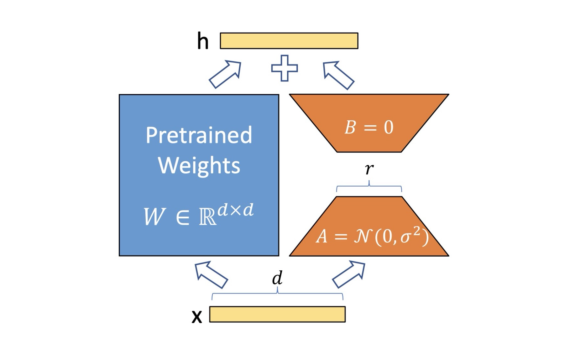
Contents
- Introduction
- Refresher on Rank of a Matrix
- Visual guide to rank(M)
- What is Low Rank Adapter?
- Brief
- Training: LoRA
- Inference: LoRA
- What does LoRA unlock?
- No Additional Latency
- Massive Storage Savings
- Dynamic Task Switching
- LoRA and a small neural network
- Experimental Setup
- The Reality of Training Large Models
- Had to freeze first 12/22 layers to fit in memory
- The Dramatic Difference
- Memory Reality Check
- Choosing the Right Rank
- End note
- References
Introduction
LoRA or Low Rank Adaptation is one of the techniques which was introduced to train large language model efficiently. To quote it in numbers, using this technique while training GPT3 175B number of trainable parameters can be reduced by 10000x, all while keeping the performance at par or better than fully finetuned model. In this blog i try to condense multiple resources and the nuances that come with this technique.
Refresher on Rank of a Matrix
Some basics first before diving into the concept. Number of linearly independent rows or columns in a matrix is known as rank of the matrix. I like to think of this in a 3D system, where each row is a vector.
Visual guide to rank(M)
Example 1:
What is the simplest 3D system that would be linearly independent? Identity matrix
Though this matrix is made of 9 numbers it's information lies across 3 dimensions. In the following representation we can clearly see each vector is linearly independent of each other.
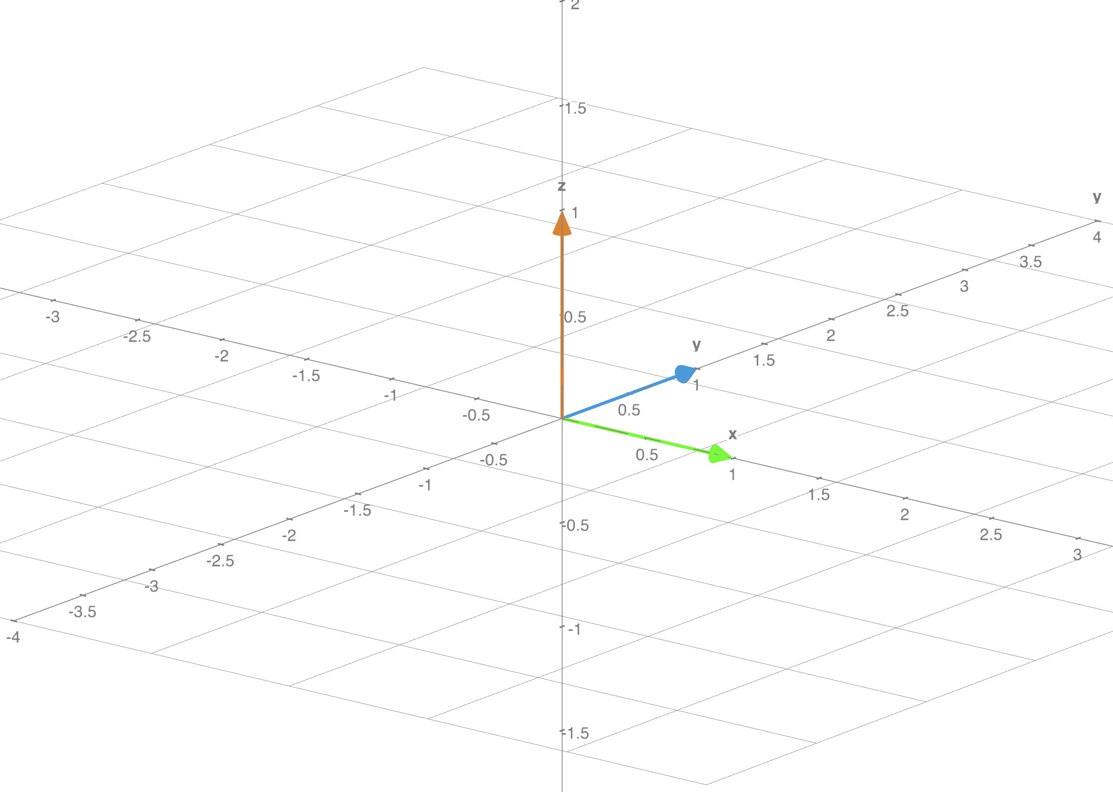
- Rank of this matrix is 3
- No row can be expressed as a linear combination of the other rows
Example 2:
Similarly a set of linearly dependent vectors looks like this:
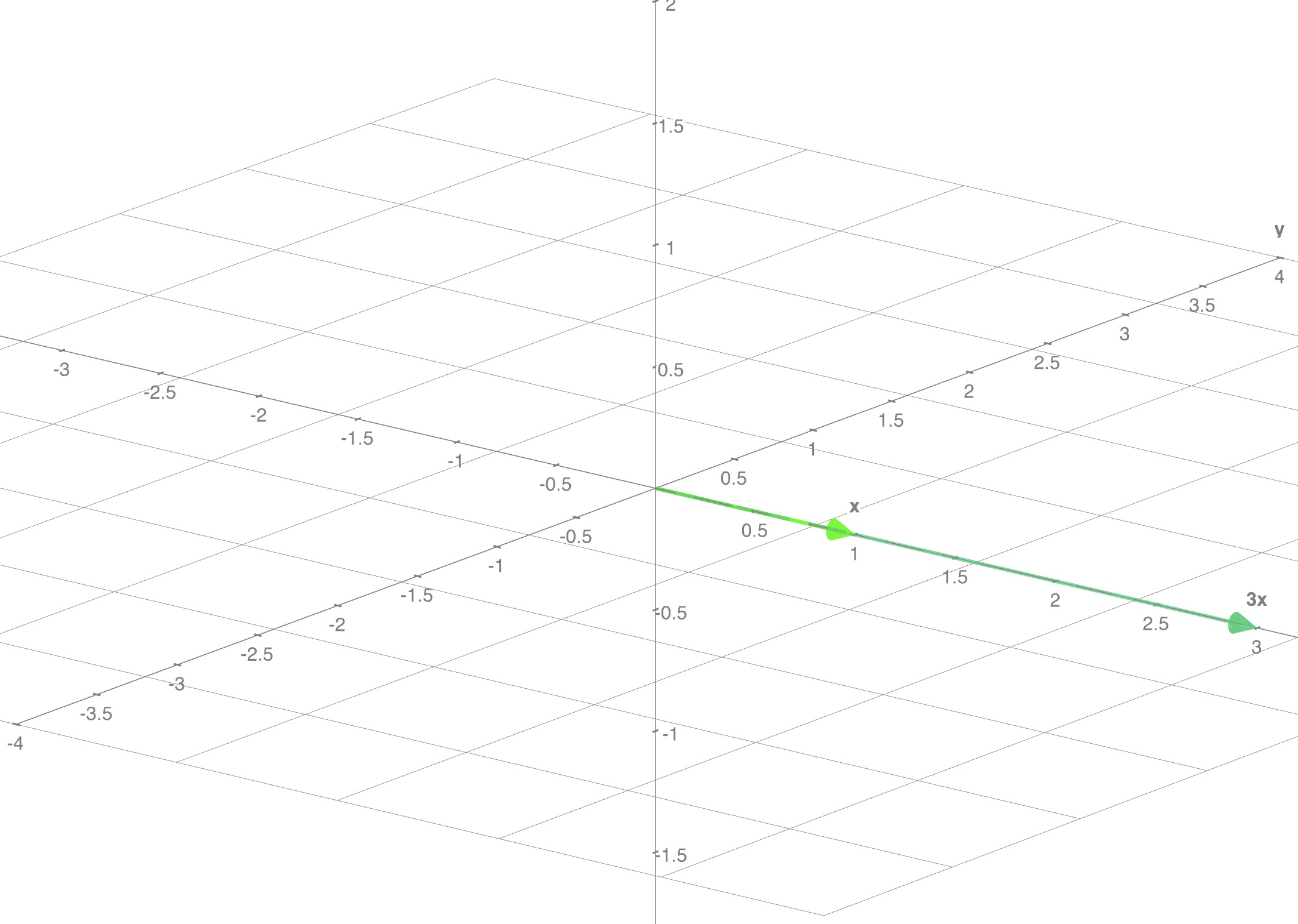
- Rank of this matrix is 1
- Row is 3 times Row
Example 3:
Extending the same concept further we can have a matrix with rank 2:
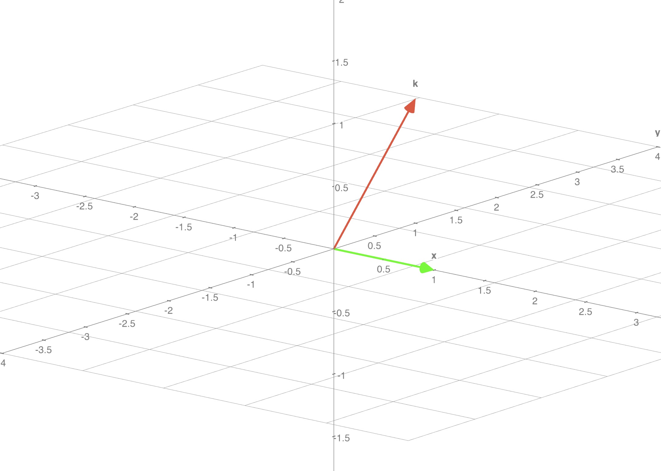
- Rank of this matrix is 2
- Only the first two rows are linearly independent, the third row is zero
Key Properties of Matrix Rank:
| Property | Mathematical Expression | Description |
|---|---|---|
| Upper bound | Rank cannot exceed smallest dimension | |
| Full vs Low rank | Full: | When rank equals smallest dimension |
| Multiplication | Product rank is bounded by minimum | |
| Addition | Sum rank is bounded by sum of ranks | |
| Subtraction | Difference rank follows same bound as addition | |
| Transpose | Rank is preserved under transpose | |
| Zero rank | Only zero matrix has rank zero |
What is Low Rank Adapter?
Brief
LoRA adds a low-rank update to frozen pre-trained weights. Instead of updating the original weight matrix directly, LoRA keeps it frozen and learns a low-rank decomposition to adapt the model:
Where:
With (r much smaller than d), making the adaptation parameter-efficient.
Essentially we are trying to learn what should be added to existing weights of a model to learn / adapt to a new task.
Visually it looks like this:
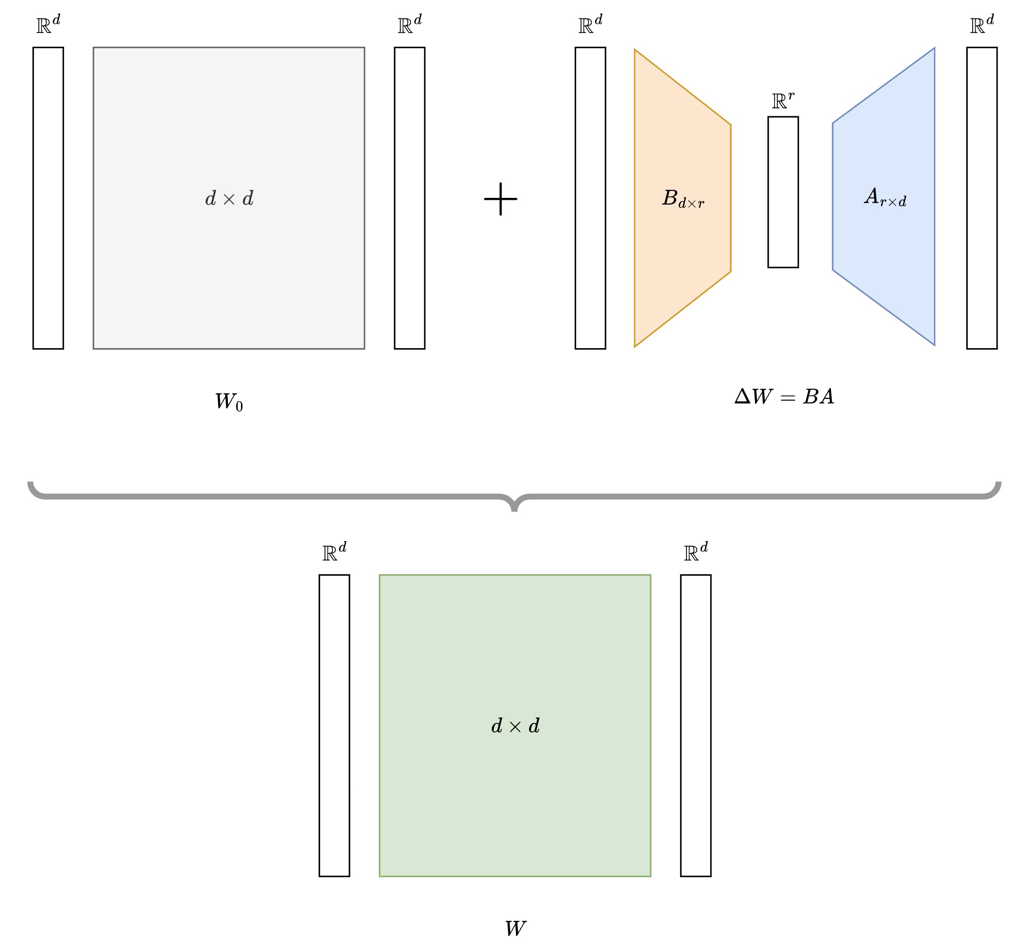
Where does rank fit in?
- Notice i.e rank in above diagram
- You choose it as a parameter, generally
- Typically , and is decided empirically
But how does it imply parameter efficient training?
- Without LoRA, learnable weights were
- With LoRA, we only need to learn weights
- As it reduces number of trainable parameters drastically
Is Rank calculated during this process?
- NO! rank of matrix is not calculated during LoRA training or inference
- When you choose hyperparameter , you are essentially saying that your matrix or will have lower rank than the original matrix
- Upon multiplication matrices and resultant rank will be which will be smaller than
- Key takeaway: You have a rank constraint, you do NOT compute it.
What does rank determine?
- How much compression you get
- How much expressivity you retain
- How much computation you save
Training: LoRA
During training:
- remains frozen (gradients blocked)
- Only and matrices are updated via backpropagation
- Forward pass: where is input
Visual guide to training LoRA
Key insight: The means gradients for are blocked/not calculated. remains completely frozen during training - only the small matrices and receive gradient updates. The dotted arrow shows this blocked gradient flow.
Inference: LoRA
During inference:
- Option 1: Compute once and use merged weights
- Option 2: Keep separate and compute
- Adapter swapping: Replace with different adapters for different tasks
Option 1: Merged Weights
Pre-compute the combined weights once, then use standard inference
Option 2: Separate Computation
Compute base and LoRA paths separately, then add their outputs
Option 3: Adapter Swapping
Keep multiple task-specific LoRA adapters and swap them dynamically
todo: - write about scaling factor and why it is important - how it is initializedWhat does LoRA unlock?
LoRA's flexible inference approaches enable several powerful capabilities:
No Additional Latency
(Option 1: Merged Weights)
- Once weights are merged (), inference runs at original speed
- No additional latency introduced during inference
- Perfect for production deployment where speed matters
Massive Storage Savings
- Store one base model + multiple small adapters instead of full fine-tuned models
- Example: Instead of storing 10 different 7B models (70GB total), store 1 base model (7GB) + 10 LoRA adapters (~50MB each = 500MB)
- Result: 70GB → 7.5GB (90% storage reduction)
Dynamic Task Switching
(Option 3: Adapter Swapping)
- Keep multiple LoRA adapters in memory simultaneously
- Switch between tasks instantly without reloading models
- Diffusion model example:
- Same base Stable Diffusion model
- Adapter 1: Anime character style
- Adapter 2: Oil painting style
- Adapter 3: Photorealistic portraits
- Switch styles in real-time based on user preference
LoRA and a small neural network
Let's look at LoRA in action with real experiments on Llama 3.2 1B model. I conducted systematic experiments to demonstrate LoRA's effectiveness compared to traditional fine-tuning approaches.
Experimental Setup
- Model: meta-llama/Llama-3.2-1B (1.24B parameters)
- Task: Sentiment analysis on IMDB dataset
- Hardware: NVIDIA A10 (23GB VRAM)
- Comparison: Baseline vs LoRA fine-tuning
The Reality of Training Large Models
Baseline Approach (Frozen Layers):
# Had to freeze first 12/22 layers to fit in memory
for param in model.model.layers[:12].parameters():
    param.requires_grad = False

Total parameters: 1,235,818,498
Trainable parameters: 505,960,450 (40.9%)
Batch size: 16 (maximum possible)
Test Accuracy: 87.16%
LoRA Approach:
lora_config = LoraConfig(
    r=16,                    # Rank
    lora_alpha=32,          # Scaling factor
    lora_dropout=0.1,       # Regularization
    target_modules=["q_proj", "v_proj", "k_proj", "o_proj",
                   "gate_proj", "up_proj", "down_proj"]
)

Total parameters: 1,247,090,690
Trainable parameters: 11,276,290 (0.9%)
Batch size: 16 (same as baseline, but could go higher)
Test Accuracy: 93.84%
The Dramatic Difference
| Metric | Baseline | LoRA | Improvement |
|---|---|---|---|
| Trainable Params | 505M (40.9%) | 11M (0.9%) | 97.8% reduction |
| Test Accuracy | 87.16% | 93.84% | +6.68% |
| Parameter Efficiency | 0.0017/M | 0.0832/M | 48.3x better |
Memory Reality Check
When I tried true full fine-tuning (all 1.24B parameters):
⚠️ CUDA OutOfMemoryError: Tried to allocate 64.00 MiB
   Even with batch size 2 - FAILED on 23GB GPU!
Meanwhile, LoRA succeeded with 8x larger batch size (16):
✅ Peak Memory: 20.57GB
✅ Training successful with much larger batches
Key insight: LoRA doesn't just make training more efficient - it makes training possible where full fine-tuning fails.
Choosing the Right Rank
The rank is a crucial hyperparameter that controls the parameter-performance trade-off.
| Rank | Use Case | Trade-off |
|---|---|---|
| Simple tasks, maximum efficiency | May underfit complex tasks | |
| Sweet spot for most tasks | Good balance | |
| Complex tasks requiring more capacity | More parameters, still efficient | |
| Very complex tasks | Approaching diminishing returns |
Rule of thumb: Start with , increase if underfitting, decrease if overfitting or need more efficiency.
End note
This brings us to the end of our deep dive into LoRA, from mathematical foundations to hands-on experiments.
But why did i cover this topic? While i was Claud-ing to research about LoRA, an interesting statement was passed by the model:
"The Manifold Hypothesis states that real-world high-dimensional data lie on low-dimensional manifolds embedded within the high-dimensional space."
It got me thinking, where else can we see this principle in action?
- Facial landmarks: 68 key points capturing the essence of infinite facial expressions
- Image embeddings: Millions of pixels compressed into meaningful feature vectors
- LoRA adapters: Complex model adaptations expressed through low-rank decompositions
All of these suggest that meaningful changes often happen in lower-dimensional spaces embedded within high-dimensional ones. LoRA's effectiveness might be capturing this fundamental property of how neural networks actually adapt and learn. Beautiful, isn't it?
All the experiments discussed in this blog have been open-sourced at https://github.com/sagarsrc/lora-experiments/ for you to reproduce and explore further.
I hope you enjoyed this blog. Have fun learning!
References
- LoRA: Low-Rank Adaptation of Large Language Models
- What is Low-Rank Adaptation (LoRA) | explained by the inventor
- LoRA - The Diet Pill for Obese Language Models
- LoRA Experiments Repository