Introduction

In the Part 1 of this series on BLT, we discussed about some prerequisites to understand Byte Latent Transformer. To summarize, BLT is a tokenizer-free architecture that matches tokenizer-based LLM performance at scale. We also saw how entropy-based patching converts the input text into a sequence of bytes.

Recall

In the last post we converted the input text into a sequence of bytes. Let’s recall the steps:

1. The input sentence was: "Sherlock Holmes is a smart detective."
2. Using entropy-based patching, we broke the sentence into patches of bytes.
3. As seen in the figure below, the sentence was broken into patches using 4 variants of entropy-based patching.

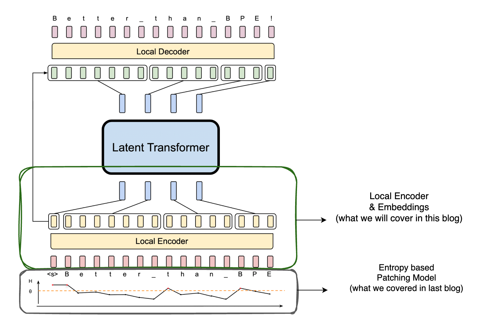
What are we going to cover today?

In this post, we will discuss about how these patches are further processed in BLT. Let us have a look at the architecture of BLT and see which areas we are going to cover in this post.

Embeddings

Once we have the patches from the entropy-based patching, we pass them through the local encoder. To get to the local encoder we need to convert the patches into embeddings first. BLT uses 3 major types of embeddings in the play here:

1. Byte Embeddings
2. Hash n-gram Embeddings
3. Position Embeddings

Let us see this in a rough flow diagram to understand it better.

Let us look deeper into each of these embeddings.

Byte Embeddings

This embedding is the simplest one. It is just a representation of all possible individual byte values which are learnt during the training of the model. For the sake of understanding the next sections, let us denote byte embeddings with $x_i$.

Hash n-gram Embeddings

Let’s try to understand how ngram embeddings work first, then we will see how and why hashing is used a bit later in this section. Instead of passing all the bytes directly to the model, we pass it in chunks, these chunks are generated exhaustively from the input text using ngrams. Let’s see how this is done.

Step 1: Basic Building Blocks

Let’s use a familiar input sentence: "Hello World"

First, let’s see what our text looks like as bytes (similar to how a computer sees it):

1H    e    l    l    o    _    W    o    r    l    d
272   101  108  108  111  32   87   111  114  108  100

Step 2: Creating Groups (N-grams)

Now comes the fun part - we’ll look at this text in different-sized windows:

For 2-letter Groups (n=2):

 1He (72,101)
 2el (101,108)
 3ll (108,108)
 4lo (108,111)
 5o_ (111,32)
 6_W (32,87)
 7Wo (87,111)
 8or (111,114)
 9rl (114,108)
10ld (108,100)

It’s like sliding a two-character window across our text!

For 3-letter Groups (n=3):

1Hel (72,101,108)
2ell (101,108,108)
3llo (108,108,111)
4lo_ (108,111,32)
5o_W (111,32,87)
6_Wo (32,87,111)
7Wor (87,111,114)
8orl (111,114,108)
9rld (114,108,100)

Now we’re looking at three characters at a time!

Step 3: ID Assignment

Here’s where it gets interesting! We give each unique group a number (like a catalog ID):

 12-letter groups:
 2"He" -> 1
 3"el" -> 2
 4"ll" -> 3
 5"lo" -> 4
 6...
 7
 83-letter groups:
 9"Hel" -> 1
10"ell" -> 2
11"llo" -> 3
12...

BLT uses ngrams of size $n$ where $n \in \{3,4,5,6,7,8\}$ .

Step 4: Hashing

Let us understand what hashing is in brief first. Hashing is like creating a fingerprint for data - it converts data of any size into a fixed-size value.

 1# X mod N = remainder
 2
 3# hash function
 4def hash_function(number, table_size):
 5    return number % table_size
 6
 7# Example
 8number = 456
 9table_size = 10
10hash_value = hash_function(number, table_size)
11
12# Output
13print(f"{number} hashes to {hash_value}")
14# 456 hashes to 6
15# 6 is the hash value

If we provide several, say 10 or 100 or even 1000 digits to the hash function, the hash value will be a single digit. Hence, we can reduce the size of the data to a single digit. But, you see the problem here is that the hash value is not unique. For example, if we have two numbers 456 and 1456, they both hash to 6. This is where the hashing function fails, this is called a collision. By increasing the complexity of the hash function, we can reduce the number of collisions and map the data to a unique hash value.

Now that we have some understanding of hashing, let us see how it is used in BLT.

Remember we are using ngrams of size 3, 4, 5, 6, 7, 8. Each of these has a different size by default. How do we map these ngrams to a unique hash value? That’s where hashing comes into the picture, it helps us create a catalog of ngrams.

This is very analogous to having a token_id for each token in the tokenizer. Instead of using the tokenizer, we are using ngrams to create a catalog of ngrams, which is then used to create embeddings. Also, because we are operating on bytes, this ngram is called as bytegrams.

Instead of using sum(ascii) % 10 as hash function, BLT uses a more sophisticated hash function to create the catalog of ngrams. The function is called as RollPolyHash (Rolling Polynomial Hash).

Taken from the paper:

Given a byte $n$-gram $g_{i,n} = {b_{i-n+1},\ldots,b_i}$

Here $g_{i,n}$ is the set of bytegrams for each byte position $i$ and $n$ from 3 to 8. $b_i$ = byte at position i

The rolling polynomial hash of $g_{i,n}$ is defined as:

$$ \text{Hash}(g_{i,n}) = \sum_{j=1}^n b_{i-j+1}a^{j-1} \qquad\dotsb\qquad (1) $$

Where $a$ is chosen to be a 10-digit prime number.

The same can be simplified as: $$\text{Hash}(g) = b_{1} + b_{2}a + b_{3}a^2 + \cdots + b_{n}a^{n-1}$$

Hash Function and Calculation of Hash Values

Formula for generating n-gram

Formula for generating n-gram: $g_{i,n} = {b_{i-n+1}, …, b_i}$

Steps:

1. Start from the current position i
2. Look back (n-1) positions from i
3. Include all elements from that starting point up to position i

Example for n-gram generation

 1# A, B, C, D, E - string
 2# 65, 66, 67, 68, 69 - byte values
 3# Showing g_{i,n} for each n-gram where i is the current position and n is the n-gram size
 4
 5g = {
 6   # 3-grams (n=3)
 7   "3_grams": {
 8       "ABC" : [65, 66, 67],  # g_{3,3}
 9       "BCD" : [66, 67, 68],  # g_{4,3}
10       "CDE" : [67, 68, 69]   # g_{5,3}
11   },
12
13   # 4-grams (n=4)
14   "4_grams": {
15       "ABCD" : [65, 66, 67, 68],  # g_{4,4}
16       "BCDE" : [66, 67, 68, 69]   # g_{5,4}
17   },
18
19   # 5-grams (n=5)
20   "5_grams": {
21       "ABCDE" : [65, 66, 67, 68, 69]  # g_{5,5}
22   },
23
24   # 6-grams (n=6)
25   "6_grams": {
26       # None possible - string length < 6
27   },
28
29   # 7-grams (n=7)
30   "7_grams": {
31       # None possible - string length < 7
32   },
33
34   # 8-grams (n=8)
35   "8_grams": {
36       # None possible - string length < 8
37   }
38}

For each of the ngram byte values, we will apply the hash function to get the hash value denoted as $h_{i,n}$.

$\text{Hash}(g_{i,n}) = b_{1} + b_{2}a + b_{3}a^2 + \cdots + b_{n}a^{n-1}$

$\text{Hash}(g_{3,3}) = 65 + 66a + 67a^2 = h_{3,3}$

$\text{Hash}(g_{4,3}) = 66 + 67a + 68a^2 = h_{4,3}$

$\text{Hash}(g_{5,3}) = 67 + 68a + 69a^2 = h_{5,3}$

…

$\text{Hash}(g_{5,5}) = 65 + 66a + 67a^2 + 68a^3 + 69a^4 = h_{5,5}$

Where $a$ as mentioned earlier is a 10-digit prime number.

But what does this hash function have to do with embeddings?

Step 5: Embeddings and Hash function

Let us see how embeddings come into the picture now.

Taken from the paper:

$$ e_i = x_i + \sum_{n=3,…,8} E_n^{hash}(Hash(g_{i,n})) \qquad\dotsb\qquad (2) $$****

I hope equation (2) seems less scary. Once we have the hash values, we can use them to get corresponding embeddings from the hash embedding table.

Here, $e_i$ is the embedding for the $i^{th}$ byte, $x_i$ is the byte embedding, $E_n^{hash}$ is the hash embedding table for the $n$-gram, and $Hash(g_{i,n})$ is the hash value for the $n$-gram.

To summarize this section pictorially:

Position Embeddings

This is used for positional reference of the input chunk of bytes, in this case instead of tokens, but the reason for using this is the same as that of position encodings in transformers. For more on that read my previous blog here. It should give you a fair understanding of what positional encodings are and why they are used in transformers.

The only difference is that BLT uses Rotary Positional Embedding (RoPE), which is a different type of positional encoding.

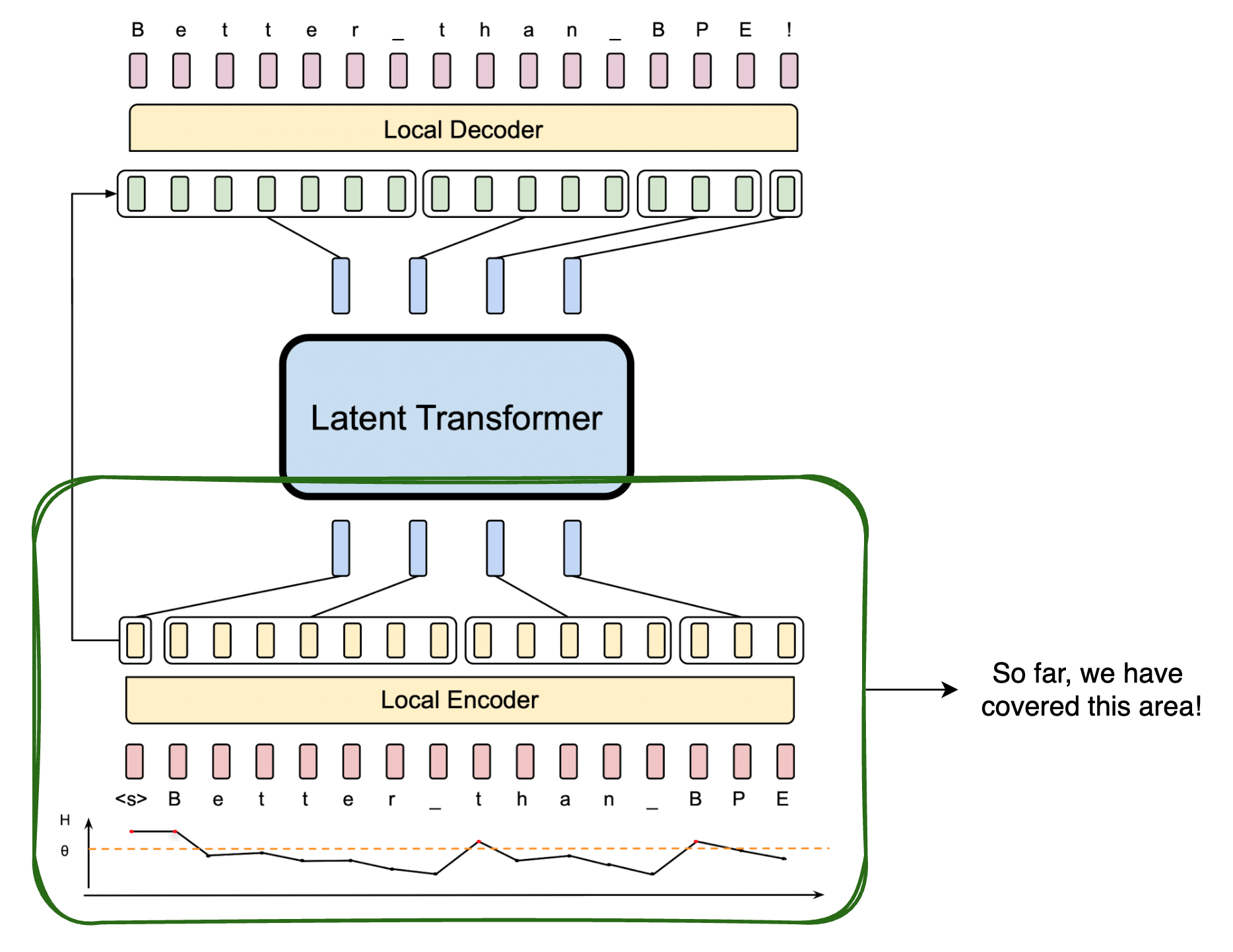
Local Encoder ($\mathcal{E}$)

Let us denote the local encoder as $\space\mathcal{E}$. The local encoder is a lightweight transformer model whose outputs are then passed to the latent global transformer model denoted as $\space\mathcal{G}$.

But where are Patches?

It’s time we ask this question. Remember in the last blog we read about patching and how we convert the input text into a sequence of bytes. So far we were only dealing with input bytes, but now let us see how we use patches to get patch embeddings.

• $n$ : number of bytes
• $p$ : number of patches
• $d$ : embedding dimension
• $p^\prime$ : downsampled output of local encoder’s hidden states
• $l_\mathcal{E}$ : number of layers in local encoder
• $l_\mathcal{G}$ : number of layers in global transformer

In the above diagram, we are essentially converting byte space to patch space, and the number of bytes is greater than the number of patches, hence $n > p$. Additionally, because the local encoder has significantly less number of layers than the global transformer ($l_\mathcal{E} \ll l_\mathcal{G}$), initial processing of bytes in the local encoder is lightweight, and compressed information is passed on to the global transformer which is computationally expensive.

Local Encoder & Attention

Let us now dive a bit deeper into how attention works in the local encoder and try to understand what are queries, keys and values in this context.

We get queries from patch space, keys and values are derived from the outputs of the local encoder. Let us pictorially look at how these are used in the local encoder to get attention scores.

Here, $a_{m,n}$ denotes the attention score for the $m^{th}$ patch and $n^{th}$ byte.

• In the case of tokenizer-based attention, this matrix would have been a square matrix (self-attention) with several rows and columns being equal to the number of patches.
• Here we have a rectangular matrix (cross attention) reason being number of patches is less than the number of bytes.
• This is cross attention as we are using patches as queries and local encoder hidden states as keys and values, two different spaces.
• We apply a masking operation to ensure that patches do not attend to bytes that are to be predicted next (area sketched in red in the above figure).
• Once we have the attention scores $(QK^T)$, we do a scaled softmax, which is later multiplied by $V$ to get the final attention output.

• All weight matrices are colored in yellow.
• Arrows moving into weight matrices denote matrix multiplications between weight matrices and incoming input matrix.
• [M] denotes projection matrix multiplications and usage of residual connections (skipping detail in the diagram for brevity).
• Final attention outputs are of the same dimension as the input embeddings, which is $(p^\prime \times d)$.
• Another important thing to note here is that we use encoder hidden states as a residual connection (More on residual connection later).

End Note

We have covered a lot of ground in this post. Let us summarize what we have covered so far:

1. How we convert the input text into a sequence of bytes (in part 1 of this series).
2. How we convert the bytes into embeddings.
3. How we use the local encoder to get attention scores and get cross attention.

Most importantly, we have seen how BLT uses a lightweight local encoder to compress information and pass it on to the latent global transformer model, this is the key reason for BLT’s significant performance gains over tokenizer-based models.

Progress Report!

In the next post, we will see how the global transformer and the local decoder work to generate the final output. We are nearing the end of this series, so stay tuned!

References

1. Byte Latent Transformer Research Paper
2. Byte Latent Transformer Github

Written By

Sagar Sarkale